syntR Tutorial
Kate Ostevik and Kieran Samuk
2019-04-17
syntr_tutorial.Rmd![]()
What is syntR?
syntR is an R package for identifying synteny blocks shared between two genetic maps. The core algorithm implemented in the package focuses on identifying synteny blocks via comparison of marker orders (e.g. from genetic maps of different species or populations). syntR identifies synteny blocks using a clustering algorithm tuned to the linear nature of genetic map data and generates an annotated list synteny block membership for each marker. syntR does not identify segmental duplications.
Requirements
syntR requires marker positions (chromosome and map position for each marker) from two genetic maps. The marker orders in the two maps need to be separately inferred for each map prior to using syntR. If you need to build you maps prior to using syntR, we reccomend looking into R/qtl, ASMap, and Lep-MAP.
Input File
The input file has six columns. Each row represents the map position of a single marker (e.g. a SNP, a microsatillite, etc.) in two different maps.
| map1_name | map1_chr | map1_pos | map2_name | map2_chr | map2_pos |
|---|---|---|---|---|---|
| HanXRQChr12_10463750 | Ann12 | 23.33200 | HanXRQChr12_10463750 | Pet12_16 | 0.000000 |
| HanXRQChr12_10463069 | Ann12 | 23.33091 | HanXRQChr12_10463069 | Pet12_16 | 3.660274 |
| HanXRQChr12_67274477 | Ann12 | 51.14234 | HanXRQChr12_67274477 | Pet12_16 | 3.660274 |
| HanXRQChr12_11545866 | Ann12 | 25.01880 | HanXRQChr12_11545866 | Pet12_16 | 3.660274 |
| HanXRQChr12_11545707 | Ann12 | 25.01856 | HanXRQChr12_11545707 | Pet12_16 | 3.660274 |
| HanXRQChr12_9937279 | Ann12 | 22.47337 | HanXRQChr12_9937279 | Pet12_16 | 4.567248 |
The columns contents are as follows:
- map1_name: A unique identifier for the marker. In this case, the markers are named based on where they reside in the sunflower reference genome (determined by aligning GBS reads).
- map1_chr: The chromosome on which the marker resides in the first map
- map1_pos: The map position (e.g. in cM) of the marker in the first map
- map2_name: As above, but for map2. These could be identical to the map1_names, or not, depending on your marker classification scheme.
- map2_chr: The chromosome on which the marker resides in the second map
- map2_pos: The map position of the marker in the second map
Example Workflow
Below, we work through an example using genetic map data from two sunflower species. Note that some of the details and tuning parameters will require tailoring to your specific maps.
1. Load and format the map data
We begin by loading the example data:
# install the package if needed!
# devtools::install_github("ksamuk/syntR")

# load the syntR package
library("syntR")

# load the example marker data
data(ann_pet_map)
as_tibble(ann_pet_map)
#> # A tibble: 1,063 x 6
#>    map1_name          map1_chr map1_pos map2_name         map2_chr map2_pos
#>    <fct>              <fct>       <dbl> <fct>             <fct>       <dbl>
#>  1 HanXRQChr12_10463… Ann12       23.3  HanXRQChr12_1046… Pet12_16     0
#>  2 HanXRQChr12_10463… Ann12       23.3  HanXRQChr12_1046… Pet12_16     3.66
#>  3 HanXRQChr12_67274… Ann12       51.1  HanXRQChr12_6727… Pet12_16     3.66
#>  4 HanXRQChr12_11545… Ann12       25.0  HanXRQChr12_1154… Pet12_16     3.66
#>  5 HanXRQChr12_11545… Ann12       25.0  HanXRQChr12_1154… Pet12_16     3.66
#>  6 HanXRQChr12_99372… Ann12       22.5  HanXRQChr12_9937… Pet12_16     4.57
#>  7 HanXRQChr12_33608… Ann12        9.06 HanXRQChr12_3360… Pet12_16     4.57
#>  8 HanXRQChr12_13257… Ann12       27.4  HanXRQChr12_1325… Pet12_16     7.22
#>  9 HanXRQChr12_17054… Ann12       32.0  HanXRQChr12_1705… Pet12_16    12.6
#> 10 HanXRQChr12_17071… Ann12       32.0  HanXRQChr12_1707… Pet12_16    12.6
#> # … with 1,053 more rows

# read in list of chromosome lengths for map1
# this is an optional file that defines the maximum
# length of each chromosome (in cM) if this is known
# NB: this is useful when the markers being compared
# do not cover the entire map

data(ann_chr_lengths)
ann_chr_lengths
#>   map1_chr map1_max_chr_lengths
#> 1    Ann08                63.68
#> 2    Ann09                96.46
#> 3    Ann12                71.68
#> 4    Ann15                80.29
#> 5    Ann16               103.49
#> 6    Ann17                97.14

# make_one_map places all the markers on a single scale
# and adds padding between the chromosomes
# to aid the algorithm and for visualization purposes
map_list <- make_one_map(ann_pet_map, map1_max_chr_lengths = ann_chr_lengths)
make_one_map outputs a list object containing three elements: - [[1]]: the marker data file with 2 additional ordering columns - [[2]] and [[3]]: the locations of the chromosome breaks between map 1 and map 2
2. Reordering the map
We can use plot_maps() to create a basic dot plot of our marker data:
# plot map
plot_maps(map_df = map_list[[1]], map1_chrom_breaks = map_list[[2]], map2_chrom_breaks = map_list[[3]])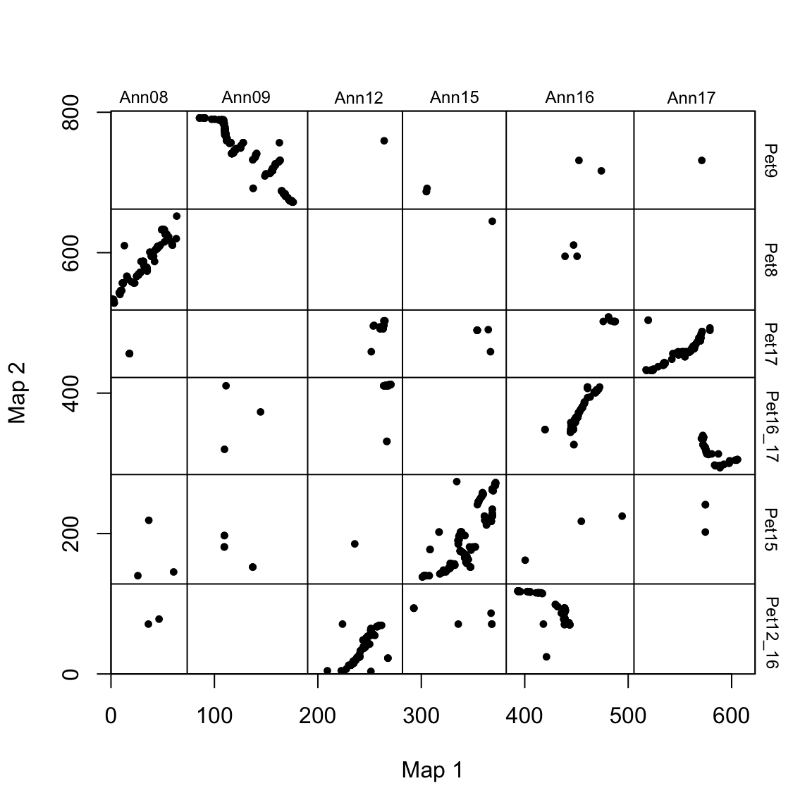
The chromosomes are annotated with their species-specific names, an the chromosome breaks are indicated by vertical and horizontal lines.
Notice that the maps look rather scattered. This is because the chromosomes are ordered arbitrarily (there is no inherent order to chromsomes). Top aid readability, we can reorder the order of chromosomes of species 2 to match the order in species 1 (plotted along the x-axis). We also rotate any “wholly-inverted” chromosomes so that they line up (at the chromosome scale) along the 1:1 line.
# reorder and flip some chromosomes
map2_chr_order <- c("Pet8", "Pet9", "Pet12_16", "Pet15", "Pet16_17", "Pet17")
flip_chrs <- c("Pet9")
map_list <- make_one_map(ann_pet_map, map1_max_chr_lengths = ann_chr_lengths, map2_chr_order = map2_chr_order, flip_chrs = flip_chrs)
plot_maps(map_df = map_list[[1]], map1_chrom_breaks = map_list[[2]], map2_chrom_breaks = map_list[[3]])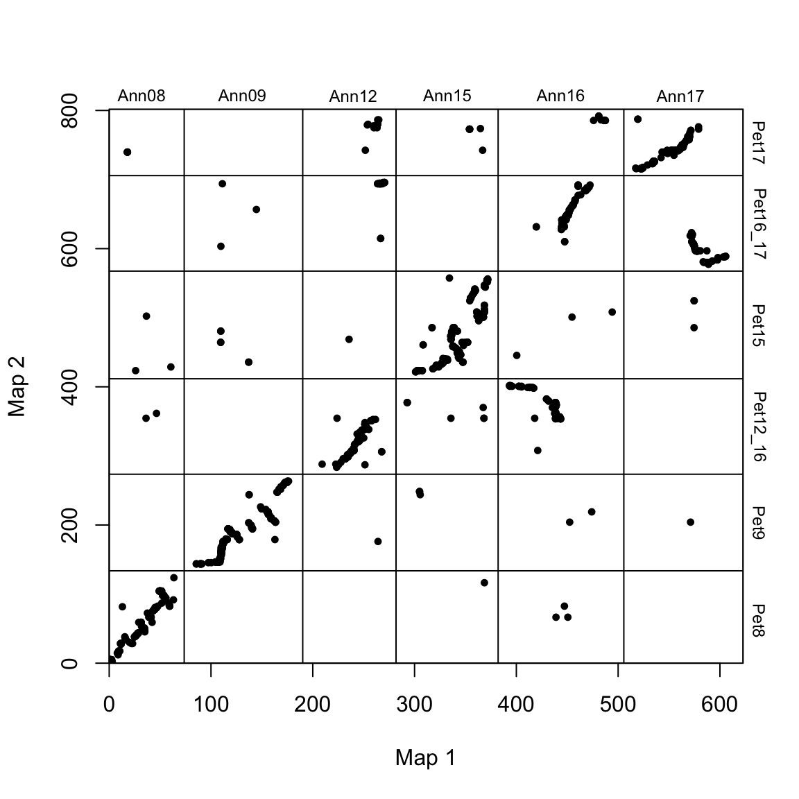
This results in a more sane-looking dot plot. However, there are clearly some translocations (e.g. Pet12_16 x Ann16) that do not conform to the 1:1 line.
3. Determine optimal turning parameters
The key tuning parameters of the syntR algorirthm are max_cluster_range and, to a lesser extent, max_nn_dist. max_cluster_range determines the maximum size of clusters of markers that will be collapsed to a singe point for further analysis. It defines the maximum distance that clustered markers can span. Lager values of max_cluster_range will result in more markers being collapsed into a single point.
max_nn_dist determines which markers are considered outliers and removed from further analysis. Markers that do not have a neighbour within max_nn_dist are considered outliers. Larger values of max_nn_dist will result in fewer markers being removed.
A simple method of finding the optimal combination of these two parameters is to fit a range of values for both and choose values that maximize coverage (% of the map assigned to synteny blocks) of the two maps and minimizes the number of outliers (“composite” in the plot below is a scaled sum of these metrics).
We provide an internal method for achieving this below. Note it is slightly computationally intensive and may take several minutes to complete.
If you’d like to skip this step, the default values of max_cluster_range = 2 and max_nn_dist = 10 are likely well suited to most genetics maps.
# find best parameter combination
# run find_synteny_blocks with each parameter combination and collect summary statistics

parameter_data <- test_parameters(map_list, max_cluster_range_list = seq(1, 5, by = 0.5), max_nn_dist_list = seq(10, 50, by = 10))
plot_summary_stats(parameter_data[[1]], "composite")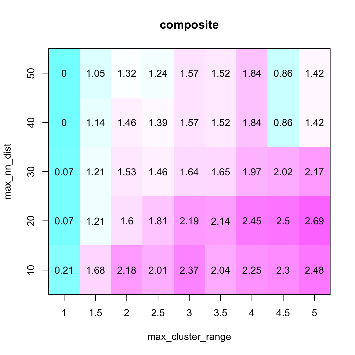
We choose the first (from left to right) composite coverage “peak” in the parameter matrix (see Ostevik et al. for details about this choice).
So, in this case, we select a max_cluster_range of 2 and a max_nn_dsit of 10.
4. Identify synteny blocks
With the two tuning parameters determined, we can run the primary function of syntR: find_synteny_blocks().
This function runs a set of marker data (contained in the map_list object we created previously) through the syntR error-detection and synteny block identification algorithm described in the Ostevik et al. publication.
It can be run as follows:
# find synteny blocks
synt_blocks <- find_synteny_blocks(map_list, max_cluster_range = 2, max_nn_dist = 10, plots = TRUE)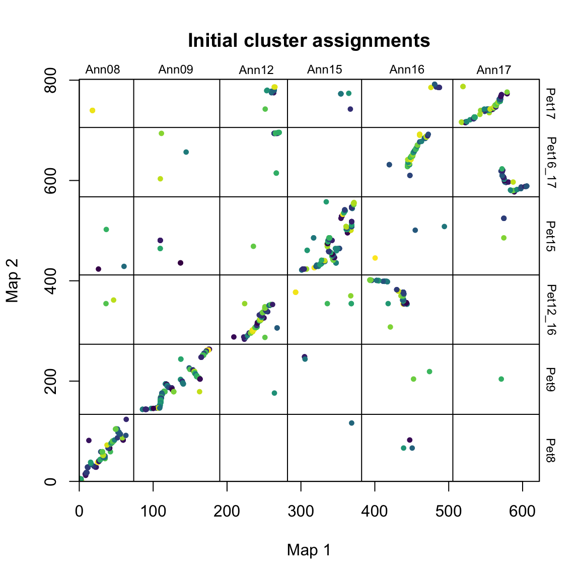
#> Warning: Factor `block` contains implicit NA, consider using
#> `forcats::fct_explicit_na`

#> Warning: Factor `block` contains implicit NA, consider using
#> `forcats::fct_explicit_na`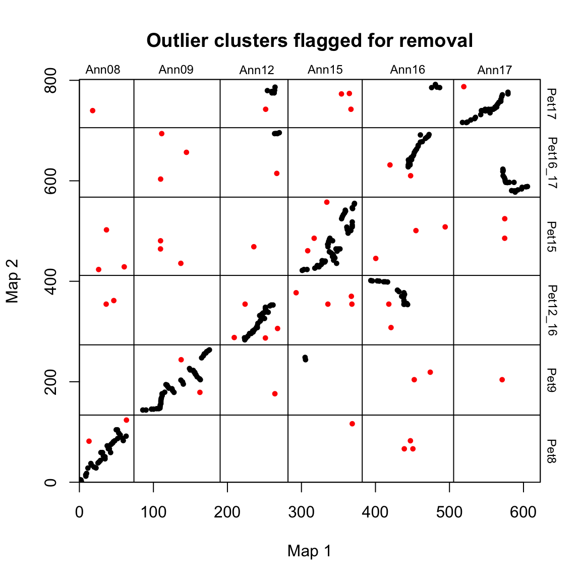
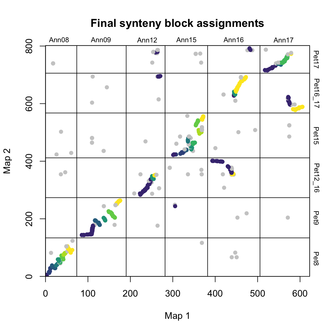
When plots=TRUE, the function generates three plots showing the progress of the algorithm. In the first plot, mapping error is smoothed via a pre-clustering step. Next, outliers are flagged and removed. Finally, synteny blocks are identified via the syntR friends-of-friends clustering algorithm.
find_synteny_blocks() outputs a list object with containing five data frames:
# print the contents of synt_blocks

lapply(synt_blocks, as_tibble)
#> $marker_df
#> # A tibble: 1,173 x 12
#>    map1_name map1_chr map1_pos map1_posfull map2_name map2_chr map2_pos
#>    <fct>     <fct>       <dbl>        <dbl> <fct>     <fct>       <dbl>
#>  1 HanXRQCh… Ann12       23.3          223. HanXRQCh… Pet12_16     0
#>  2 HanXRQCh… Ann12       23.3          223. HanXRQCh… Pet12_16     3.66
#>  3 HanXRQCh… Ann12       51.1          251. HanXRQCh… Pet12_16     3.66
#>  4 HanXRQCh… Ann12       25.0          225. HanXRQCh… Pet12_16     3.66
#>  5 HanXRQCh… Ann12       25.0          225. HanXRQCh… Pet12_16     3.66
#>  6 HanXRQCh… Ann12       22.5          223. HanXRQCh… Pet12_16     4.57
#>  7 HanXRQCh… Ann12        9.06         209. HanXRQCh… Pet12_16     4.57
#>  8 HanXRQCh… Ann12       27.4          228. HanXRQCh… Pet12_16     7.22
#>  9 HanXRQCh… Ann12       32.0          232. HanXRQCh… Pet12_16    12.6
#> 10 HanXRQCh… Ann12       32.0          232. HanXRQCh… Pet12_16    12.6
#> # … with 1,163 more rows, and 5 more variables: map2_posfull <dbl>,
#> #   cluster <int>, block <fct>, final_block <int>, orientation <chr>
#>
#> $synteny_blocks_df
#> # A tibble: 41 x 8
#>    block map1_chr map1_start map1_end map2_chr map2_start map2_end
#>    <fct> <fct>         <dbl>    <dbl> <fct>         <dbl>    <dbl>
#>  1 5     Ann08         0.308     3.10 Pet8            0       5.87
#>  2 6     Ann08         7.97     11.6  Pet8           12.1    28.4
#>  3 7     Ann08        15.4      23.0  Pet8           28.4    38.2
#>  4 8     Ann08        24.9      28.6  Pet8           38.2    43.6
#>  5 9     Ann08        32.6      34.8  Pet8           48.0    50.7
#>  6 10    Ann08        29.1      32.6  Pet8           51.6    59.1
#>  7 11    Ann08        37.5      42.2  Pet8           59.1    72.5
#>  8 12    Ann08        42.7      47.8  Pet8           75.2    82.6
#>  9 14    Ann08        51.1      63.1  Pet8           82.6   104.
#> 10 29    Ann09         1.96     28.6  Pet9            0      32.4
#> # … with 31 more rows, and 1 more variable: orientation <chr>
#>
#> $map1_breaks
#> # A tibble: 35 x 2
#>     start    end
#>     <dbl>  <dbl>
#>  1   3.10   7.97
#>  2  11.6   15.4
#>  3  23.0   24.9
#>  4  28.6   29.1
#>  5  32.6   32.6
#>  6  34.8   37.5
#>  7  42.2   42.7
#>  8  47.8   51.1
#>  9 112.   117.
#> 10 128.   137.
#> # … with 25 more rows
#>
#> $map2_breaks
#> # A tibble: 35 x 2
#>     start   end
#>     <dbl> <dbl>
#>  1   5.87  12.1
#>  2  28.4   28.4
#>  3  38.2   38.2
#>  4  43.6   48.0
#>  5  50.7   51.6
#>  6  59.1   59.1
#>  7  72.5   75.2
#>  8  82.6   82.6
#>  9 176.   179.
#> 10 194.   194.
#> # … with 25 more rows
#>
#> $summary_stats
#> # A tibble: 1 x 4
#>   num_blocks map1_coverage map2_coverage n_outliers
#>        <int>         <dbl>         <dbl>      <int>
#> 1         41          383.          567.        205
These elements are:
$marker_dfA data frame including the original list of markers along with their synteny block assignments.$synteny_blocks_dfA data frame summarizing the span of each synteny block in each map (in map units) along with their inferred orientation (colinear, inverted, etc.) for synteny blocks with sufficient evidence of directionality.$map1_breaksA data frame listing the breakpoints between synteny blocks in map1.$map2_breaksA data frame listing the breakpoints between synteny blocks in map2.$summary_statsA data frame summarizing the results of the algorithm (coverage etc.)
We can plot the blocks with their orientation as below:
# plot synteny block orientations
synt_blocks[[1]] %>%
    plot_maps(map_list[[2]], map_list[[3]], col = c("blue", "grey", "red", "black")[as.numeric(as.factor(.$orientation))],
              main = "Synteny block orientation",  cex_val = 0.75)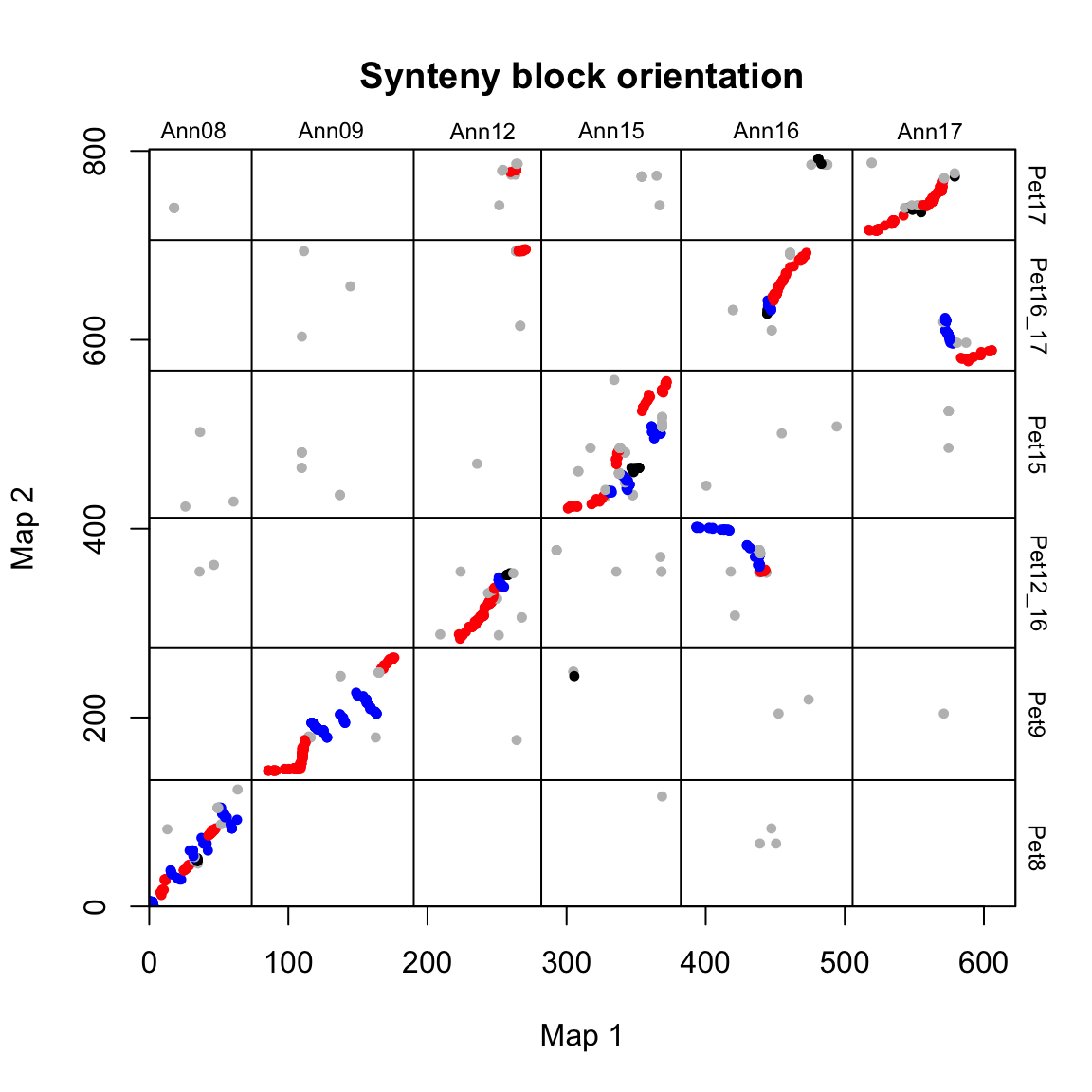
In this case, blue = inverted, red = colinear and grey/black = unclassified.